PyTorch深度学习实践Part4——反向传播
对于简单模型可以手动求解析式,但是对于复杂模型求解析式几乎不可能。
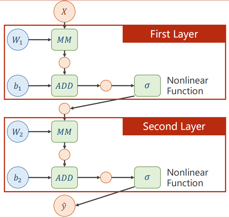
计算图
每一层神经网络包括一次矩阵乘法(Matrix Multiplication)、一次向量加法、非线性变化函数(为了防止展开函数而导致深层神经网络无意义)
链式法则
在pytorch中,梯度存在变量而不是计算模块里。
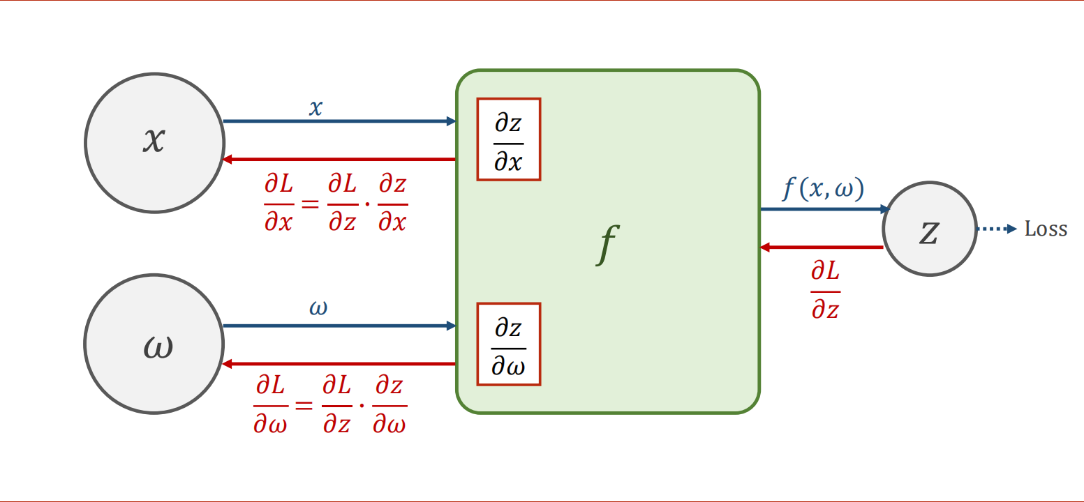
在计算过程中中,虽然有些变量可以不求导,但是一样要具备能够求导的能力。比如x的值就有可能是前一层网络的y_hat传递下来的。
核心在于梯度,loss虽然不会作为变量参与计算过程,但是同样需要保留,作为图像数据来判断最终是否收敛。
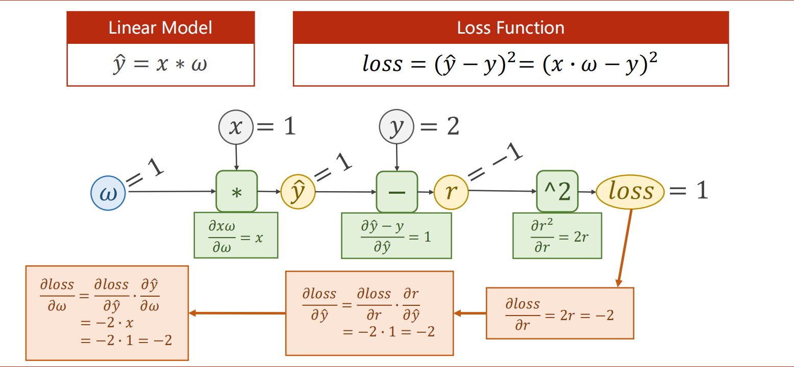
PyTorch实现反向传播
线性模型y=w*x,用pytorch实现反向传播
1
2
3
4
5
6
7
8
9
10
11
12
13
14
15
16
17
18
19
20
21
22
23
24
25
26
27
28
29
30
31
32
33
34
| import torch
x_data = [1.0, 2.0, 3.0]
y_data = [2.0, 4.0, 6.0]
w = torch.Tensor([1.0])
w.requires_grad = True
def forward(x):
return x * w
def loss(x, y):
y_pred = forward(x)
return (y_pred - y) ** 2
print("predict (before training)", 4, forward(4).item())
for epoch in range(100):
for x, y in zip(x_data, y_data):
l = loss(x, y)
l.backward()
print('\tgrad:', x, y, w.grad.item())
w.data = w.data - 0.01 * w.grad.data
w.grad.data.zero_()
print('progress:', epoch, l.item())
print("predict (after training)", 4, forward(4).item())
|
课后作业
二次模型y=w1x²+w2x+b的反向传播
1
2
3
4
5
6
7
8
9
10
11
12
13
14
15
16
17
18
19
20
21
22
23
24
25
26
27
28
29
30
31
32
33
34
35
36
37
38
39
40
41
| import torch
x_data = [1.0, 2.0, 3.0]
y_data = [4.0, 9.0, 16.0]
w1 = torch.Tensor([1.0])
w2 = torch.Tensor([1.0])
b = torch.Tensor([1.0])
w1.requires_grad, w2.requires_grad, b.requires_grad = True, True, True
def forward(x):
return w1 * x * x + w2 * x + b
def loss(x, y):
y_pred = forward(x)
return (y_pred - y) ** 2
print("predict (before training)", 4, forward(4).item())
for epoch in range(100):
for x, y in zip(x_data, y_data):
l = loss(x, y)
l.backward()
print('\tgrad:', x, y, w1.grad.item(), w2.grad.item(), b.grad.item())
w1.data = w1.data - 0.01 * w1.grad.data
w2.data = w2.data - 0.01 * w2.grad.data
b.data = b.data - 0.01 * b.grad.data
w1.grad.data.zero_()
w2.grad.data.zero_()
b.grad.data.zero_()
print('progress:', epoch, l.item())
print("predict (after training)", 4, forward(4).item())
print(w1.data, w2.data, b.data)
|
改了一下原本的数据集,更符合二次函数,但是因为样本量过少,预测的权重并不是很好。