1
2
3
4
5
6
7
8
9
10
11
12
13
14
15
16
17
18
19
20
21
22
23
24
25
26
27
28
29
30
31
32
33
34
35
36
37
38
39
40
41
42
43
44
45
46
47
48
49
50
51
52
53
54
55
56
57
58
59
60
61
62
63
64
65
66
67
68
69
70
71
72
73
74
75
76
77
78
79
80
81
| import numpy as np
import matplotlib.pyplot as plt
x_data = [1.0, 2.0, 3.0]
y_data = [5.0, 8.0, 11.0]
def forward(x):
return x * w + b
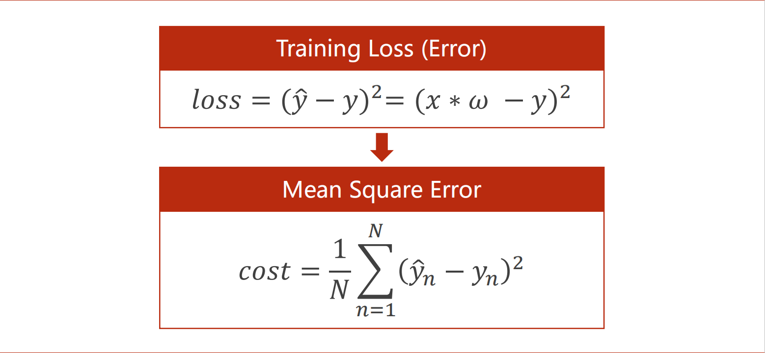
def loss(x, y):
y_pred = forward(x)
return (y_pred - y) * (y_pred - y)
w_list = np.arange(0.0, 4.1, 0.1)
b_list = np.arange(0.0, 4.1, 0.1)
w, b = np.meshgrid(w_list, b_list)
l_sum = 0
for x_val, y_val in zip(x_data, y_data):
y_pred_val = forward(x_val)
loss_val = loss(x_val, y_val)
l_sum += loss_val
print('\nx_val:', x_val,'\ny_val:', y_val, '\ny_pred_val:',y_pred_val, '\nloss_val:',loss_val)
mse_list = l_sum / 3
print('MSE=', mse_list)
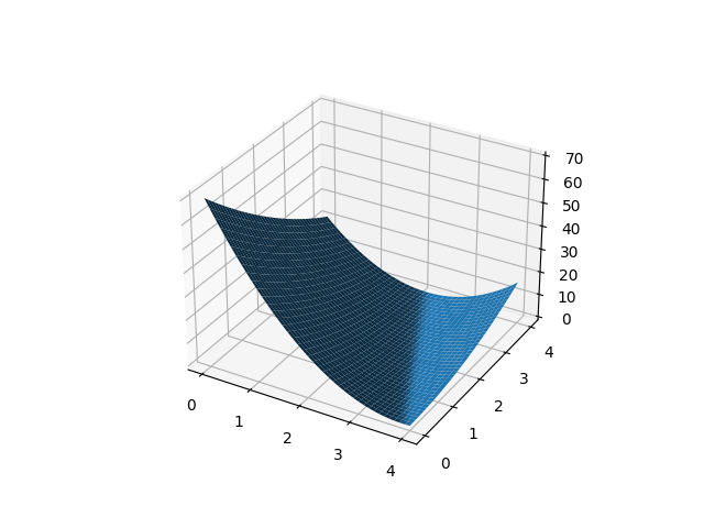
fig = plt.figure()
ax = fig.add_subplot(111, projection='3d')
ax.plot_surface(w, b, mse_list)
plt.show()
import numpy as np
import matplotlib.pyplot as plt
x_data = [1.0, 2.0, 3.0]
y_data = [5.0, 8.0, 11.0]
def forward(x):
return x * w + b
def loss(x, y):
y_pred = forward(x)
return (y_pred - y) * (y_pred - y)
w_list = np.arange(0.0, 4.1, 0.1)
b_list = np.arange(0.0, 4.1, 0.1)
w, b = np.meshgrid(w_list, b_list)
l_sum = 0
for x_val, y_val in zip(x_data, y_data):
y_pred_val = forward(x_val)
loss_val = loss(x_val, y_val)
l_sum += loss_val
print('\nx_val:', x_val,'\ny_val:', y_val, '\ny_pred_val:',y_pred_val, '\nloss_val:',loss_val)
mse_list = l_sum / 3
print('MSE=', mse_list)
fig = plt.figure()
ax = fig.add_subplot(111, projection='3d')
ax.plot_surface(w, b, mse_list)
plt.show()
|